Wednesday 3 May 2023

What will YOU do about Climate Change?

 We have a climate emergency but individuals might feel they can make little difference. Here are some suggestions:  

  • Protest: Governments normally follow public opinion rather than lead.  We need to let all levels of government (and large companies) know that more action is required (such as banning new coal and gas, putting a price on carbon, better incentives for electrification, removing fossil fuel subsidies etc etc).  Protesting can take many forms, including writing letters, joining demonstrations, using social media. Beware of green washing.  
  • Educate: Humanity has a number of challenges at present, but Climate Change is probably the biggest.  Mainstream media consistently understates the problem.  Check some of the references below and then talk with your family, friends, social groups, work colleagues, sports clubs etc to explain the seriousness of the climate emergency. 
  • Support: If you can afford it, please support and/or donate to organisations that are trying to make a difference, for example The Australia Institute, Australian Greens, Renew Economy. This might include moving your investments and savings (superannuation, shares, bank accounts) from fossil fuel supporters to greener options.   
  • Conserve: Trying to reduce your own carbon footprint is a step in the right direction and provides an example to others.  This will make an increasing difference as more people do it.  Examples include: recycle where possible, ditch gas appliances, buy an EV (bike or car), eat less meat,  insulate your home, turn down the air con,  convert to a heat-pump for hot water,  review travel plans. 

Some motivations for Climate Action: 
Johan Rockstrom's Earth Day 2023 Message (6 minute YouTube video) 
National Centre for Climate Restoration (Breakthrough web site) 
"The 2084 Report: A History of Global Warming from the Future"  (novel by James Powell)
National Centre for Climate Restoration (Breakthrough) 
National Centre for Climate Restoration (Breakthrough) National Centre for Climate Restoration (Breakthrough) 

Thursday 3 November 2022

More Bee Hive Telemetry


Spring is a busy time for bees and bee keepers.  In a previous post I described some simple measurements of our bee hives that help confirm the queen is producing new brood and the bees are active.  Recently I added a weighing device to a hive in our garden with the aims of a) seeing the hive weight gradually increasing over the period of peak honey production and b) detecting a swarming event by a sudden drop in hive weight.  


In summary the additional electronics consists of 4 strain gauges plus an HX711 interface chip that converts the the differential signal from the strain gauges to a 24 bit digital value, which is then fed via a serial interface to the existing Pro-Mini micro-controller and LoRa radio system.  A swarm is detected by checking for a drop in hive weight by at least 500 gm over about 30 minutes.  When this happens the system sends me an SMS.   

This picture shows the bee hive with brood box and super sitting on the hive "scales".  I used 4 low-cost strain gauges from E-bay, typically employed in bathroom scales. One is located under each corner of the hive.  The black cable entering the rear of the brood box goes to a thermistor in the "brood ball" and gives the blue signal in the plot below.  The green plot is the external temperature.  The white box contains the micro-controller and LoRa radio.  


I was not expecting to see many swarms detected by additional electronics, but unfortunately we've had two in the last month!  The first weight plot shows a pretty dramatic drop (over 2 kg).  This "primary swarm" happens when the old queen leaves, with a significant fraction of the colony.  It went into a neighbour's tree and I was able to capture it and start a new hive.


  The time scales of the temperature and weight plots overlap and it's interesting to see (before the swarm) that the hive weight is increasing more rapidly during some warmer weather.  This Spring in Adelaide has been unusually wet and cold. 


A secondary swarm occurred yesterday. It was smaller in number of bees and the weight drop is also less. The weight reduction is not just the bee weight - they eat lots of honey before leaving for sustenance while finding a new home. This swarm went into another neighbour's garden and was easy to catch.  I gave these bees to an apiarist in the Bee Soc. of SA. We are fortunate to have very understanding neighbours!   

Friday 7 May 2021

Satellite Orbits from their Doppler Trajectories?

Summary

This post explores possibilities for estimating satellite orbits based on Doppler variations of their signals over time.  Selected orbits parameters have been estimated  using the Python's SciPy optimisation library.  Initial experiments have been promising but more remains to be done. 

Background

There are many useful applications of the Doppler effect.  I found this recent example particularly interesting in the use of Doppler measurements to detect exoplanets.   

Some years ago I was trying detect low earth orbit (LEO) satellites in the radio amateur bands by looking for their characteristic Doppler profile.  As a satellite approaches a ground station (GS) its radio signal frequency appears higher, while overhead there's no frequency offset, and as it recedes the carrier frequency continues to drop.  Several satellites can be seen in the "waterfall" plot below, with time increasing from top to bottom and frequency from left to right. The vertical scale is 60 minutes but the plot superimposes results from a few hours.  Although this spectrum region is dedicated to radio amateur satellites, there are often sources of terrestrial interference which obscure the small satellite signals,  so part of the task is to automatically remove the non-satellite signals (a few remnants can still be seen below).   In addition the spectral width of LEO signals varies,  so a filtering and median tracking approach has been used to only estimate the carrier frequency.   

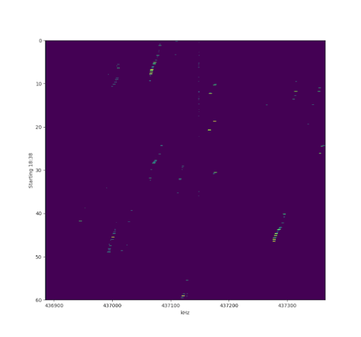
Showing spectral signatures of several LEO satellites in the 70 cm band, over 60 minutes. 
 
An Orbit Estimation Experiment. 

 While the "blind" detection of LEO satellites is interesting in its own right, this post asks whether some orbital parameters can be estimated just using their Doppler shapes.  Doppler shift is proportional to the satellite's velocity in the direction of the GS, so overhead passes show greater Doppler variations than low elevation passes.  Initially I assumed it would be possible to estimate the minimum distance from the GS to the satellite and perhaps it's orbital height.  Many LEO satellites have almost circular orbits and I've made that assumption below.  In addition it seemed likely that collecting the same signal from two different locations might provide information regarding orbit inclination. During the investigations I realised that the Earth's motion must be taken into account,  which provides some additional possibilities, even for one GS. 

Others have used Doppler measurements to refine existing orbit estimates, which are usually disseminated by the TLE standard.  Mark alerted me to the strf software and I changed my data collection format to use their file standard.  So far I've used signals collected from two satellites, by myself and Mark.  On April 16th we each recorded a pass from LUSAT (LO-19) and FalconSat-3. Both of these provide relatively strong continuous downlink transmissions, and they use different orbits and signal characteristics.  The figure shows a summary of the satellite passes used.  These GSs are located near Adelaide and are almost 90 km apart.  


The figure below used the strf code and shows one of the FalconSat-3 signals.  In this case the signal bandwidth is significant and I've written some Python code to implement a simple comb filter to track the carrier frequency.  


Given a set of carrier frequency measurements over several minutes, plus an orbit model with unknown parameters, it's a non-trivial problem to estimate the orbital unknowns.  Fortunately SciPi provides a versatile library function to address this type of problem.    My model uses the following unknowns: time offset, frequency offset, angle between GS and the satellite's crossing of the equator, orbit height and orbit offset from 90 degrees inclination.  

The figure below shows an example of Doppler measurements and fitted Doppler trajectory.   The blue points are automatically extracted from a selected portion of the raw strf file which contains spectral estimates from a simple RTL2832 software defined radio, connected to a low gain antenna.  The orange curve represents the modelled trajectory after the MSE optimisation.  In this case the estimated orbit height of 487 km was quite accurate, plus the time of minimum range when compared to TLE predictions using gpredict. 


FalconSat-3 Path Estimate 

LUSAT Path Estimate 

Also shown is the model's estimated path in 3D of FalconSat-3 (blue dots) relative to the GS (yellow X). In both cases a red marker shows the last time position.  Note this path illustrates a descending node pass (i.e. moving away from the equator in green), like the figure above.  When the satellite direction in the model was assumed to be ascending, the fitted solution was poor.  The model didn't make a good prediction of inclination - ~45 degrees compared to 35 actual.  In the LUSAT case, the minimum range estimate was accurate to within a few km, but the orbit height was quite poor (1109km compared to about 790 km).  In this case the ascending model gave a slightly better fit than the descending node model.   

Conclusions 

At times the Doppler trajectory seems able to give surprisingly accurate orbit estimates. Note that the sample recordings used strong signals and captured more of the trajectory than a low SNR pass would provide.  In the near-polar LUSAT case, with similarly good data, the results are not so close and seem somewhat dependent on the initial estimates given to the estimator.  Perhaps this is not surprising given the non-linear nature of the model and the reduced affect of GS motion compared to a non-polar orbit.  A simpler model, without inclination, seems to give robust results but doesn't provide as much information. This MSE solver has many parameters options and I've barely scratched the surface in its use.  

The original idea of using two GS recordings from the same pass hasn't been explored in any detail. I expect a larger distance separation will be needed to get useful results.  A model which jointly fits (say) the frequency difference between the two signals is likely to work better than making separate estimates then combining the results.  In addition, at present the signal strength measurements are not used at all! The use of (say) two antennas (whose gain patterns are known), pointed in different directions at one GS,  might open many other options for orbit estimation.  


Thursday 12 November 2020

Climate Solutions are Possible!

This post is about an excellent climate modelling tool called En-ROADS,  developed by MIT and other organisations.  By using a "hands-on" approach, it allows individuals or groups to learn about those factors producing climate change and also how to best to address the climate crisis.  I haven't included any sample graphics - it's better if you explore the link above. You might start with the 3 minute video demo of how it works, then try running your own model.


This is what I like about En-ROADS:  

  • Tackling climate change is tricky. Leaving aside factors such as the influence of vested interests and biased media, climate modelling requires physical, economic and social models, with a high degree of interaction between the parameters. For example, given a price per ton on carbon, how will this affect CO2 emissions and then what is the impact on mean temperature over future decades?   How does this strategy compare to (say) a tax of coal?   En-ROADS actually answers these questions, plus a great deal more.  
  • Are the models accurate?  It's reassuring that En-ROADS has been compared to many other climate models and IPCC standard scenarios (called SSPs) - it seems to give quite consistent results.  There's a lot of good climate science behind the software, and it's being regularly updated. 
  • This tool is freely accessible to the public via a simple http web page.  With so many input and output parameters the user interface it critical.  En-ROADS provides a set of the most important adjustment levers (eg adjust how much of the transport system is electrified, assume a higher or lower population growth, adjust taxes on oil etc) then shows the resultant effect on mean temperature increase, compared to "business as usual".  However there's a wealth of other results that can be displayed, plus detailed settings that can be adjusted.  This degree of transparency and detailed modelling is wonderful - it's necessary to capture the complexity, but also might be daunting for casual users.   En-ROADS therefore suggests a guided approach eg in an interactive workshop format.  

Is En-ROADS perfect?  It's scope is already very broad, so it's not surprising that some aspects can not be included.  For example
  • A global, rather than regional, model is assumed so it represents a global mean of climate policies and their results.  Note some other tools on the Climate Interactive site look into various regional issues. 
  • In general, tipping points are hard to model, plus the interaction between these positive feedback loops.   Thus in some respects En-ROADS may be too optimistic, depending on the values of various assumptions used in the model.  At least En-ROADS provides useful information, plus references,  regarding its assumptions.  
  • En-ROADS predicts outcomes such as CO2 concentrations over time, sea level rise, mean temperature increase etc.  The "business as usual" path shows over 2 degrees temperature rise by mid century and about 4 degrees by 2100.  Of course 4 degrees will probably result in catastrophic outcomes for humanity.  At present it's too hard to model the effect of this on (say) GDP. 
Summary

En-ROADS allows users to explore climate mitigation strategies in order to understand drivers and discover the most promising approaches.   It's well designed and implemented, with a lot of detailed information if users want to explore specific areas.  It also includes many examples and includes a focus on equitable carbon-neutral transformations.  

En-ROADS suggests it's possible to avoid a climate disaster via a suitable mix of strategies.  However it's not easy to achieve (say) less than two degrees average temperature rise and there's certainly no single quick fix.  

----------------------------------------

"Dealing with Climate Change" U3A Workshop:   May 2021   


Wednesday 7 October 2020

Checking on the Bee Hive

Temperature, humidity and other parameters of bee hives can be measured and provide useful indications of hive status and health.   Here is one example of commercially-available equipment.   

So during the last year I've been monitoring our bee hive.  A Lora system sends telemetry from Arduino-based electronics next to the hive.  Over the last Spring and Summer the temperature regulation was extremely good - usually within one degree, whatever the weather.  During Winter the temperature was highly variable and we wondered if the hive was healthy.  The Adelaide plains are fairly easy for bees during colder months and in previous Winters we left the Super on the Brood Box, however this year we removed the Super and I added extra insulation.  Happily the bee hive looked OK during some physical inspections. 

    
Hive Temp at end of August 

We didn't need to worry.  The plot shows temperature near the middle of the Brood Box in green, plus external temperature in black, over a one week period. Towards the end of this period the variations seem to decrease and the average temperature is rising.  

Hive Temperature, start of September  

This graph follows directly from the previous.  (My simple plotting doesn't restart the day number partway through the plot, but it's the first week of September.) Amazingly the bees have begun to closely regulate the brood temperature!   From this research,  

Honeybee larvae and pupae are extremely stenothermic, i.e. they strongly depend on accurate regulation of brood nest temperature for proper development (33–36°C).


It seems remarkable that bees can do this.  As warm-blooded mammals we can regulate temperature pretty well. But the bees are doing this for their nursery area, using both active and passive methods.  Furthermore they can turn it on or off.  They don't waste energy in thermoregulation unless there are young bees to look after.  Spring is a busy time in the bee hive!   


Apart from temperature,  we've also looked at humidity in the hive. Thermistors are easy to insert into the hive compared to humidity sensors.  For a more novel experiment, I've tried to measure the level of hive activity.  Last year our hive swarmed a few times.  We managed to capture the swarms and donate them to worthy recipients, but swarming may not be ideal for the neighbours.  So it seems useful to at least know if the hive is more active than usual.  Others have used audio and even video processing methods.  I've tried sensing the bee motion in and out of the hive via light-level variations.    Light Dependent Resistors (LDRs) at either end of the hive entrance measure the instantaneous light levels, which change as bees walk by. The figure below shows typical results over 7 days.  

Hive Activity over one week


The upper plot shows the mean light level on a log scale.   LDRs have terrific dynamic range and during the dark periods (i.e. nights) they even pick up moon light!   The lower plot shows the normalised standard deviation over intervals of about 20 seconds.  The two sensors at each end of the entrance gives rise to blue and green plots, although the green is largely over-written.  You can see that bee activity varies quite a bit from day to day, as the weather changes.  Perhaps the next step will be a temperature compensated plot that provides alerts on unusual activity.  


The activity monitoring started in Winter but the LDRs had minimal protection and failed after a few months. Close inspection shows moisture ingress on the sensor surface.   The encapsulation of LDR devices probably varies considerably.  I'm hoping my current LDRs will last longer - each is encased in the end of a glass test tube to provide more protection. This image shows one end of the bridge over the hive entrance, before installation.  The upper surface sits next to the side of the hive.  


Wednesday 1 July 2020

21cm Radio Astronomy


The image above shows recent results from our 2m dish in Prospect looking at the 21 cm Hydrogen signal (with star positions superimposed).  It's plotted in galactic coordinates and represents data collected over a few months.  Red indicates H1 moving away from us; blue is Doppler shifted to higher frequencies as the H1 moves towards us.  Leaving the dish in a fixed position for one day gives a curved track as the Earth rotates. (For example the almost circular tracks in the slightly-lower right side arose when the antenna was close to the South Celestial Pole.  The Pointers and Southern Cross can be clearly seen near zero latitude.)     We did a talk on this project recently for AREG

Thursday 9 January 2020

Sun Shades to Cool the Earth?

Introduction

Given the present inadequate global response to reducing greenhouse gas (GHG) emissions, some people are considering geoengineering options to ameliorate the effects of the climate changes which we have begun to observe.  Many worry that deliberate intervention in the Earth's climate system is a bad idea since the unexpected effects could be dangerous and in addition the usual fossil fuel polluters might use this solution as a "get out of gaol" card.  The top priority should be drastic GHG reduction, but it seems prudent to explore the feasibility of geoengineering methods as backup.  Hence this page briefly reviews the idea of reducing global warming by a space-based approach of solar flux reduction.   See [1] or [2] for an introduction to geoengineering. 

Solar Flux Control 
The idea of controlling solar radiation to limit climate change effects is not new (e.g. see [3]).  Terrestrial methods of geoengineering may be cheaper, but this space-based approach has potential advantages:

  • once installed, it might be possible to adjust the attenuation fairly rapidly
  • it might offer some ability for varying the solar radiation depending on latitude.  
The figure below contains a simple 2D model of flux attenuator located near the L1 Lagrange point, a distance (L in the figure) about 1.5 million km from the Earth on the left hand side.  At this location the gravitational forces towards the Earth and the Sun are balanced, providing a pseudo-stable "parking spot".   The sun's disc is shown in the right;   it subtends an angle of about half a degree from the Earth.  We assume some type of mirror is used to block solar radiation that would otherwise fall on the Earth's surface.  (Other options such as a large thin Fresnel lens to disperse sunlight have also been proposed.)  

Fig 1:  2D Model of Solar Flux Control (not to scale) 

For realistic mirror dimensions, no part of the Earth would be fully in shadow from the mirror (i.e. the umbra doesn't extend to the earth).  An observer on Earth would not notice any change in the Sun, unless equipped with a pin-hole camera or similar. Assume that the mirror's position  can be adjusted in the vertical direction shown in Fig 1.  This allows some scope in varying the flux versus latitude on the Earth.   For example a simple evaluation using the 2D model above, with a 1000 km mirror, offset by 3000km, gives the Figure 2 reduction in flux versus position on the Earth.  In this example case the mirror is located "below" the Earth-Sun midpoint so for regions near the North Pole, no part of the Sun's disc is obstructed and the attenuation is zero.   


Fig. 2: Example of Solar Flux Reduction 
Previous studies of similar sun shades have concluded that only a few percent reduction in solar radiation might counter the GHG heating effects and have suggested mirrors of similar dimensions.  

Feasibility  
Radiation will exert a force on the mirror (solar sails use this  effect) and for (say) a 1000 km square mirror this is large (e.g. almost 8 million Newtons). However this should not pose a major problem as the structure can be placed on the Sun side of the L1 Lagrange point such that the radiation force balances the net gravitational force.  Of course second-order effects would require an active positioning system, probably provided by many small thrusters.  

The main challenge appears to be manufacture and transport of the mirror(s).  For a mirror of 1 gram per square meter, the area mentioned above requires 1 million tonnes of mirror.  Fabrication on the Earth  doesn't appear to be likely given estimates of the total mass launched into space are considerably less.   Manufacture in space seems more promising but is probably a long term project compared to the time available.  For example the moon contains a large percentage of Aluminium that might form the bulk of the reflecting material.  Some asteroids could also provide useful raw materials, such as Nickel.  If significant amounts of Aluminium could be mined and smelted on the Lunar surface, it could be used to make very thin reflecting sheets (possibly unrolled and assembled at L1) together with structural elements required for the large fleet of positioning cubesats.  Presumably the required micro-electronic components could be made on Earth, with highly automated assembly of the cubesats on the Moon and possible launch via a Space Gun

Conclusions 

Control of solar flux seems feasible but is a long term project.  All the more reason to make rapid cuts in our greenhouse gas emissions and avoid the need for these extreme measures.